[PRML] 1.2: Linear regression with L1 and L2 regularization
This is my reading notes for the book Pattern Recognition and Machine Learning by Bishop.

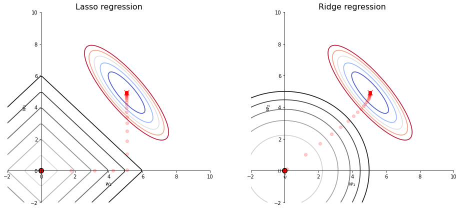
Lasso regression versus Ridge regression: Lasso regression uses L1 regularization, which tends to create sparse solution ($w_2$ equal or close to zero when $\lambda$ takes a large value); Rdige regression uses L2 regularization, which pushes both weights to zero simultanously when $\lambda$ increases.
Linear regression
Consider an D-dimensional input variable $\boldsymbol{x} = \begin{bmatrix} x_1 & x_2 & \dots & x_D \end{bmatrix}^\top$ and a scalar output variable $y$. The input-output relation between $\boldsymbol{x}$ and $y$ is unknwon.
Given a training dataset with $N$ observations ${\boldsymbol{x}_n, y_n}$, where $n = 1, \dots, N$, the goal is to predict $y$ for a new $\boldsymbol{x}$.
The linear regression model is a linear combination of $(x_1, \dots, x_D )$,
\[f(\boldsymbol{x}, \boldsymbol{w}) = w_0 + w_1x_1 + w_2x_2 + \dots + w_Dx_D = \boldsymbol{w}^\top\boldsymbol{x},\]or a linear combination of basis functions $(\phi_1(\boldsymbol{x}), \dots, \phi_M(\boldsymbol{x}))$
\[f(\boldsymbol{x}, \boldsymbol{w}) = w_0 + w_1\phi_1(\boldsymbol{x}) + w_2\phi_2(\boldsymbol{x}) + \dots + w_M\phi_M(\boldsymbol{x}) = \boldsymbol{w}^\top\boldsymbol{\phi}(\boldsymbol{x}).\]Maximum likelihood and least squares
In the previous note we have derived the least sqaure solution of linear regression:
\[\boldsymbol{w}^* = (\boldsymbol{\Phi}^\top\boldsymbol{\Phi})^{-1}\boldsymbol{\Phi}^\top\boldsymbol{y}\]Now we will approach this problem using the maximum likelihood method.
To use the maximum likelihood method, we need to assume a probabilistic model between the input $\boldsymbol{x}$ and the target output $y$. For example, a linear Gaussian model:
\[y = \boldsymbol{w}^\top\boldsymbol{\phi}(\boldsymbol{x}) + \epsilon,\]where $\epsilon \sim \mathcal{N}(0, \sigma^2)$ is the additive Gaussian noise.
The likelihood function, which describes the probability of observing ${y_n}$ given ${\boldsymbol{x}_n}$ ($n = 1, \dots, N$), is a function of parameters $\boldsymbol{x}$ and $\sigma$:
\[p(\boldsymbol{y}\ |\ \boldsymbol{X}, \boldsymbol{w}, \sigma) = \prod_{n=1}^{N} \mathcal{N}(y_n\ |\ \boldsymbol{w}^\top\boldsymbol{\phi}(\boldsymbol{x}_n), \sigma^2) = \prod_{n=1}^{N} \frac{1}{\sqrt{2\pi \sigma^2}}\exp\{ -\frac{[y_n - \boldsymbol{w}^\top\boldsymbol{\phi}(\boldsymbol{x}_n)]^2}{2\sigma^2} \}.\]The log-likelihood is often used for its simplicity:
\[\ln p(\boldsymbol{y}\ |\ \boldsymbol{X}, \boldsymbol{w}, \sigma) = -\frac{N}{2}\ln2\pi\sigma^2 - \frac{1}{2\sigma^2}\sum_{n=1}^N [y_n - \boldsymbol{w}^\top\boldsymbol{\phi}(\boldsymbol{x}_n)]^2\]At this point, it is straightforward to see that the $\boldsymbol{w}$ maximize the likelihood function is equivalent to the $\boldsymbol{w}$ minimize $\sum_{n=1}^N [y_n - \boldsymbol{w}^\top\boldsymbol{\phi}(\boldsymbol{x}_n)]^2$, which leads to the same result as the least square solution.
Note: Maximum likelihood $\neq$ least square.
- The maximum likelihood method assumes a linear Gaussian model between the input and output variables, while the least square makes no such assumption.
- It is a special case in the linear Gaussian case, the maximum likelihood method gives the same results as the least square method.
Regularized least square
The regularized least square method can be presented in the following optimization problem:
\[\min_{\boldsymbol{w}}\ || \boldsymbol{y} - \boldsymbol{w}^\top\boldsymbol{\Phi} ||^2 + \lambda ||\boldsymbol{w}||_q\]where
\[||\boldsymbol{w}||_q = (\sum_{m=1}^M |w_m|^q)^{\frac{1}{q}}\]and $\lambda$ is the regularization coefficient.
LASSO regression ($\ell_1$-norm regularization)
The LASSO regression has the following form:
\[\min_{\boldsymbol{w}}\ \sum_{n=1}^N [\boldsymbol{y} - \boldsymbol{w}^\top\boldsymbol{\phi}(\boldsymbol{x}_n) ]^2 + \lambda \sum_{m=1}^M |w_m|\]or
\[\min_{\boldsymbol{w}}\ || \boldsymbol{y} - \boldsymbol{\Phi}\boldsymbol{w} ||^2 + \lambda ||\boldsymbol{w}||\]The LASSO regression does not have analytic solutions and need to be solved computationally (see Problem 6.11 and Section “$\ell_1$-norm regularization” in the book Convext Optimization).
Below is the Python code for solving the Lasso regression with CVXPY.
# LASSO regression with CVXPY
def loss_fn(X, Y, w):
    return cp.norm2(X@w - Y)**2

def regularizer_l1(w):
    return cp.norm1(w)

def objective_fn_lasso(X, Y, w, lambd):
    return loss_fn(X, Y, w) + lambd * regularizer_l1(w)

w_lasso = cp.Variable(shape=(2,1))
lambd = cp.Parameter(nonneg=True)
problem = cp.Problem(cp.Minimize(objective_fn_lasso(X, y, w_lasso, lambd)))

for l in lambda_range:
    lambd.value = l
    problem.solve()
    w1, w2 = w_lasso.value
Ridge regression (squared Euclidean norm, also known as Tikhonov regularization)
The Ridge regression has the following form:
\[\min_{\boldsymbol{w}}\ || \boldsymbol{y} - \boldsymbol{\Phi}\boldsymbol{w} ||^2 + \lambda ||\boldsymbol{w}||^2\]which has the analytical solution
\[\boldsymbol{w}^* = (\lambda\boldsymbol{I} + \boldsymbol{\Phi}^\top\boldsymbol{\Phi})^{-1}\boldsymbol{\Phi}\boldsymbol{y}.\]