[PRML] 1.1: Polynomial Curve Fitting
This is my reading notes for the book Pattern Recognition and Machine Learning by Bishop.
Let’s reproduce the first example in the book – ploynomial curve fitting (page 4-7).
The data

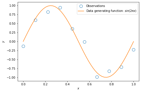
Plot of the training data: $ y = \sin(2\pi x) + \text{noise}$
The polynomial function
Fit the observations using a polynomial function of the form:
\[f(x, \boldsymbol{w} ) = w_0 + w_1 x + w_2 x^2 + ... + w_M x^M = \sum^{M}_{j=0}{w_j x^j}.\]Let $\phi_j(x) = x^j$ be the basis function, the vector form of the above polynomial function is
\[f(x, \boldsymbol{w} ) = \sum^{M}_{j=0}{w_j \phi_j(x)} = \boldsymbol{w}^\top\boldsymbol{\phi},\]where $\boldsymbol{w} = \begin{bmatrix} w_0 & … & w_M \end{bmatrix}^\top$, and $\boldsymbol{\phi} = \begin{bmatrix} \phi_0(x) & … & \phi_M(x) \end{bmatrix}^\top$
Below is the Python implementation of the above polynomial function:
def polynomial(w, x):

    # w is the (M+1,) coefficients vector
    # x is the (N,) input vector
    # y is the (N,) output vector

    N = np.size(x)
    M = np.size(w) - 1
    y = np.zeros((N,))

    for n in range(0, N):
        y[n] = np.transpose(w).dot((x[n]*np.ones((M+1,)))**range(0, M+1))

    return y
The mean square error function
Given N observations of $x$:
\[\boldsymbol{x} = \begin{bmatrix} x_1 & ... & x_N \end{bmatrix}^\top,\]and N corresponding observations of $y$:
\[\boldsymbol{y} = \begin{bmatrix} y_1 & ... & y_N \end{bmatrix}^\top,\]the mean-square error (MSE) function is
\[\text{MSE}(\boldsymbol{w}) = \frac{1}{N} \sum^{N}_{n=1}[ f(x_n, \boldsymbol{w}) - y_n ]^2,\]or in the matrix form:
\[\text{MSE}(\boldsymbol{w}) = \frac{1}{N}(\boldsymbol{\Phi}\boldsymbol{w} - \boldsymbol{y})^\top(\boldsymbol{\Phi}\boldsymbol{w} - \boldsymbol{y}),\]where
\[\boldsymbol{\Phi} = \begin{bmatrix} \phi_0(x_1) & \phi_1(x_1) & \dots & \phi_M(x_1) \\ \phi_0(x_2) & \phi_1(x_2) & \dots & \phi_M(x_2) \\ \vdots & \vdots & \ddots & \vdots \\ \phi_0(x_N) & \phi_1(x_N) & \dots & \phi_M(x_N) \\ \end{bmatrix}.\]Minimize the MSE (model fitting)
The polynomial curve fitting is done by selecting the values of the coefficients $\boldsymbol{w}$ which minimize the MSE.
Take the derivate of MSE with respect to $\boldsymbol{w}$ and let it equal to zero,
\[\frac{\partial}{\partial \boldsymbol{w}} \frac{1}{N}(\boldsymbol{\Phi}\boldsymbol{w} - \boldsymbol{y})^\top(\boldsymbol{\Phi}\boldsymbol{w} - \boldsymbol{y}) = 0\]where
\[\begin{align}\frac{\partial}{\partial \boldsymbol{w}}(\boldsymbol{\Phi}\boldsymbol{w} - \boldsymbol{y})^\top(\boldsymbol{\Phi}\boldsymbol{w} - \boldsymbol{y}) =& \frac{\partial}{\partial \boldsymbol{w}} (\boldsymbol{w}^\top\boldsymbol{\Phi}^\top - \boldsymbol{y}^\top)(\boldsymbol{\Phi}\boldsymbol{w} - \boldsymbol{y})\\ =& \frac{\partial}{\partial \boldsymbol{w}} (\boldsymbol{w}^\top\boldsymbol{\Phi}^\top\boldsymbol{\Phi}\boldsymbol{w} - 2\boldsymbol{y}^\top\boldsymbol{\Phi}\boldsymbol{w} + \boldsymbol{y}^\top\boldsymbol{y}) \\ =& 2\boldsymbol{w}^\top\boldsymbol{\Phi}^\top\boldsymbol{\Phi} - 2\boldsymbol{y}^\top\boldsymbol{\Phi} \end{align}\]Therefore the optimal coefficients $\boldsymbol{w}^*$ is
\[\boldsymbol{w}^* = (\boldsymbol{\Phi}^\top\boldsymbol{\Phi})^{-1}\boldsymbol{\Phi}^\top\boldsymbol{y}\]Below is the Python implementation of the above polynomial fitting procedure:
def polynomial_fit(x, y, M):

    # x is the (N,) input vector
    # y is the (N,) output vector
    # M is the order of the polynomial function
    # Phi is the (N, M) design matrix
    # w is the (M+1,) coefficients vector

    N = np.size(x)
    Phi = np.zeros((N, M+1))

    for m in range(0,M+1):
        Phi[:, m] = x**m

    w = np.linalg.inv(np.transpose(Phi).dot(Phi)).dot(np.transpose(Phi)).dot(y)

    return w
The over-fitting problem
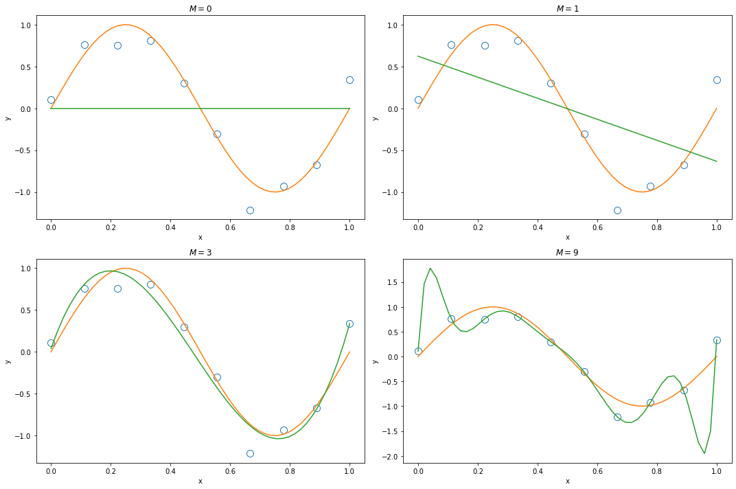
When we only have 10 observations, a high order polynomial function ($M=9$) will cause over-fitting.

Increasing the size of training data (from $N = 10$ to $N = 100$) reduces the over-fitting problem.
